Heap Structure

We previously saw that our known data structures with the best runtime for our PQ operations was the binary search tree. Modifying its structure and the constraints, we can further improve the runtime and efficiency of these operations.

We will define our binary min-heap as being complete and obeying min-heap property:

Min-heap: Every node is less than or equal to both of its children
Complete: Missing items only at the bottom level (if any), all nodes are as far left as possible.

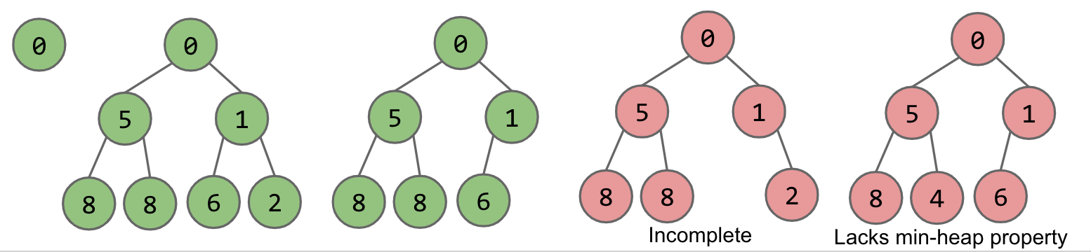
As we can see in the figures above, the green colored heaps are valid and the red ones aren't. The last two aren't because they violate at least one of the properties that we defined above.

Now let's consider how this structure lends itself to the abstract data type we described in the previous chapter. We will do this through analyzing our desired operations.

Exercise 13.2.1. Determine how each method of our Priority Queue interface will be implemented given this heap structure. Don't write actual code, just pseudocode!

Heap Operations

The three methods we care about for the PriorityQueue ADT are add, getSmallest, and removeSmallest. We will start by conceptually describing how these methods can be implemented given our given schema of a heap.

add: Add to the end of heap temporarily. Swim up the hierarchy to the proper place.
- Swimming involves swapping nodes if child < parent
getSmallest: Return the root of the heap (This is guaranteed to be the minimum by our min-heap property
removeSmallest: Swap the last item in the heap into the root. Sink down the hierarchy to the proper place.
- Sinking involves swapping nodes if parent > child. Swap with the smallest child to preserve min-heap property.

Great! We have determined how we will approach the operations specified by the PriorityQueue interface in an efficient way. But how do we actually code this?

Exercise 13.2.2. Give the runtime for each of the methods specified above. Worst cases and best cases.

Tree Representation

There are many approaches we can take to representing trees.

Approach 1a, 1b, and 1c

Let us consider the most intuitive and previously used representation for trees. We will create mappings between nodes and their children. There are several ways to do this which we will explore right now.

In approach Tree1A, we consider creating pointers to our children and storing the value inside of the node object. These are hardwired links that give us fixed-width nodes. We can observe the code:

public class Tree1A<Key> {
  Key k;
  Tree1A left;
  Tree1A middle;
  Tree1A right;
  ...
}

The visualization of this type of structure is shown below.

Alternatively, in Tree1B, we explore the use of arrays as representing the mapping between children and nodes. This would give us variable-width nodes, but also awkward traversals and performance will be worse.

public class Tree1B<Key> {
  Key k;
  Tree1B[] children;
  ...
}

Lastly, we can use the approach for Tree1C. This will be slightly different from the usual approaches that we've seen. Instead of only representing a node's children, we say that nodes can also maintain a reference to their siblings.

public class Tree1C<Key> {
  Key k;
  Tree1C favoredChild;
  Tree1C sibling;
  ...
}

In all of these approaches, we store explicit references to who is below us. These explicit references take the form of pointers to the actual Tree objects that are our children. Let's think of more exotic approaches that don't store explicit references to children.

Approach 2

Recall the Disjoint Sets ADT. The way that we represented this Weighted Quick Union structure was through arrays. For representing a tree, we can store the keys array as well as a parents array. The keys array represent which index maps to which key, and the parents array represents which key is a child of another key.

public class Tree2<Key> {
  Key[] keys;
  int[] parents;
  ...
}

Take some time to ensure that the tree on the left corresponds to the representation in the arrays on the right.

It's time to make a very important observation! Based on the structure of the tree and the relationship between the array representations and the diagram of the tree, we can see:

The tree is complete. This is a property we have defined earlier.
The parents array has a sort of redundant pattern where elements are just doubled.
Reading the level-order of the tree, we see that it matches exactly the order of the keys in the keys array.

What does this all mean? We know the parents array is redundant so we can ignore it and we know that a tree can be represented by level order in an array.

Approach 3

In this approach, we assume that our tree is complete. This is to ensure that there are no "gaps" inside of our array representation. Thus, we will take this complex 2D structure of the tree and flatten it into an array.

public class TreeC<Key> {
  Key[] keys;
  ...
}

With the continued diagram from above:

This will be our similar to the book's scheme for implementing the heap, which is the underlying implementation for the Priority Queue ADT.

Swim

Given this implementation, we define the following code for the "swim" described in the Heap Operations section.

public void swim(int k) {
    if (keys[parent(k)] ≻ keys[k]) {
       swap(k, parent(k));
       swim(parent(k));              
    }
}

What does the parent method do? It returns the parent of the given k using the representation in Approach 3.

Exercise 13.2.3. Write the parent method. For extra challenge, try to write the methods for finding the left child and right child of a given item.

13.2 Heaps